Google Sheets•5 min read
Google Sheets UNIQUE Function: Extract Distinct Values
Remove duplicates and extract distinct values in Google Sheets with the UNIQUE function. Real examples, sorting, and error fixes.
SheetHub••5 min
A customer import that lists the same buyer five times, or a column of regions repeated across a hundred rows, makes any summary count say more than it should. The Google Sheets UNIQUE function fixes this by returning a clean list of the distinct values from a range, and because it is a formula, the result recalculates the moment your source data changes. This guide covers how to use the 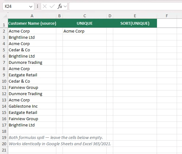
 For the cross-platform behavior of the same function, the Excel dynamic array functions guide covers the Excel equivalent,
Suppose a support log lists
Because
Often a value is unique on its own but the same combination appears more than once. A row is a duplicate only when both the customer and the region and the date match. Feed the whole row range into
This returns the distinct rows where the date is in 2026 or later. You can wrap the whole thing in
For the cross-platform behavior of the same function, the Excel dynamic array functions guide covers the Excel equivalent,
Suppose a support log lists
Because
Often a value is unique on its own but the same combination appears more than once. A row is a duplicate only when both the customer and the region and the date match. Feed the whole row range into
This returns the distinct rows where the date is in 2026 or later. You can wrap the whole thing in 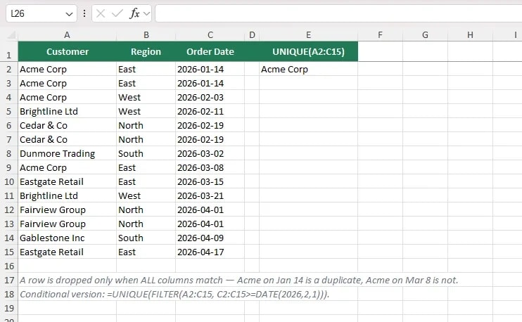 If you only need to count how many unique items exist rather than list them, the COUNTUNIQUEIFS guide shows the single-function approach for counting distinct values by criteria.
The Google Sheets UNIQUE function turns a range into a clean list of distinct values that updates itself as the data changes. Use
=UNIQUE() function in Google Sheets, step-by-step implementation patterns, and practical troubleshooting for real spreadsheets.
UNIQUE is the formula equivalent of the Data menu's Remove duplicates command, but it has one big advantage: it does not touch your source data. It just spills the distinct values into a fresh range, so the original table stays intact and the list stays in sync.
Zoom
What is UNIQUE and how does it work?
UNIQUE takes a range of values and returns only the distinct entries, dropping every subsequent repeat. By default it deduplicates by row across all the columns you give it, so a row is kept only if the whole combination is new. This is different from COUNTUNIQUEIFS, which counts distinct items instead of listing them.
Syntax
=UNIQUE(range, [by_column], [exactly_once])- range: The cells, or the range of cells, containing the values you want to deduplicate.
- by_column (optional):
TRUEto compare values column by column instead of by row. - exactly_once (optional):
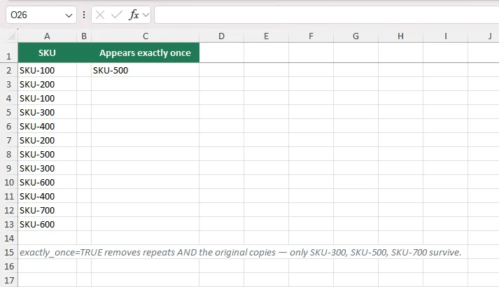
TRUEto return only values that appear exactly once, dropping every duplicated value entirely.
exactly_once argument is the part most people miss. UNIQUE(A2:A100, FALSE, TRUE) returns only items that show up exactly one time, which removes the duplicates and the original copies of anything that was repeated.
Zoom
UNIQUE, in the context of FILTER, SORT, and SEQUENCE.
Pattern 1: Build a distinct list of customers
Customer Name in column A, from A2 to A100. The same person keeps appearing because they opened several tickets. You want one clean list of customers to feed into a dropdown or a chart.
=UNIQUE(A2:A100)How this works:
UNIQUEreads every name inA2:A100.- It keeps the first occurrence of each name and drops the repeats.
- The distinct names spill down from the cell where you type the formula.
SORT:
=SORT(UNIQUE(A2:A100))SORT and UNIQUE are both dynamic array functions, they spill together and re-sort automatically whenever a name is added or removed. To turn the result into a self-updating selector for a form, this complements the Google Sheets FILTER function pattern for live reports.
Pattern 2: Extract unique rows based on multiple columns
UNIQUE and it deduplicates across every selected column.
=UNIQUE(A2:C100)How this works:
- Columns A, B, and C hold the customer, region, and order date.
UNIQUEtreats each full row as the unit of comparison.- Only truly identical rows are dropped, so two orders by the same customer on different dates both stay.
FILTER first:
=UNIQUE(FILTER(A2:C100, C2:C100 >= DATE(2026,1,1)))SORT to fix the order, and each layer recalculates as the source changes.
Zoom
Troubleshooting and common errors
| Error / Symptom | Root Cause | Practical Fix |
|---|---|---|
#REF! or #VALUE! | The range includes an empty or incompatible type, or the spill area is blocked by existing data. | Clear the cells below the formula and check that the range contains the same kind of value. |
| Duplicates still show | The values differ by invisible whitespace or leading spaces, so "Acme " and "Acme" are treated as two entries. | Wrap each text column in TRIM or clean the source first. |
UNIQUE skips a value you expected | Compare is case-insensitive, so "Apple" and "apple" count as one. | Use FILTER with EXACT for a case-sensitive result. |
| Blank rows appear at the end | Blank cells are treated as a distinct value. | Filter the range with a condition that removes blanks, such as UNIQUE(FILTER(A2:A100, A2:A100<>"")). |
| "Result overflow" message | The output touches a column that already has data. | Move the formula or the blocked data so the spill range stays empty. |
Summary
UNIQUE for a simple list, add by_column and exactly_once for edge cases, nest it with SORT or FILTER for ordered and conditional results, and keep the source data untouched so nothing is lost. Pair it with COUNTUNIQUEIFS when all you need is a count instead of a list.Recommended Next Reading
Google Sheets
=GOOGLE(...)Google Sheets COUNTUNIQUEIFS: Count Unique by Criteria
Explore ↗
Google Sheets
=GOOGLE(...)Google Sheets INDIRECT: Build Dynamic Sheet References
Explore ↗
Google Sheets
=EDATE() / =TODAY()Google Sheets SEQUENCE: Generate Numbers, Dates & Grids
Explore ↗
Share this tutorial
Discussion & Community
Share questions, tips, or edge-cases about this spreadsheet formula.